Procedure

Download the Analysis folder from the sbhs website. It will be available under downloads section. Download the file for SBHS Analysis Code (local & virtual). The name of the file is scilab_codes_analysis. The download will be in zip format. Extrat the downloaded zip file. You will get a folder scilab_codes_analysis.

Open the scilab_codes_analysis folder and then locate and open the folder Ramp_Analysis.

Copy the ramp test data file to this folder.

Change the Scilab working directory to Ramp_Analysis

Open the file ramp_virtual.sce in scilab editor and enter the name of the data file (with extention) in the filename field.

Save and run this code and obtain the plot as shown in figure 3.4.

label.sci

costf_1.sci

**Figure 3.4:** Output of the Scilab code `ramp_virtual.sce`

**Figure 3.5:** Scilab console after executing code`ramp_virtual.sce`

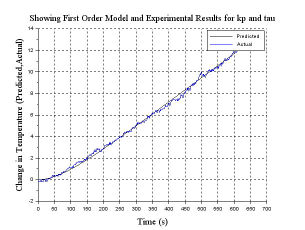
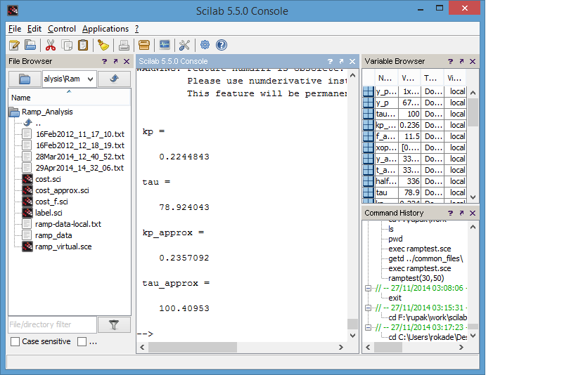
The results presented are obtained for the data file ramp-data-virtual.txt. This data file is present under the Ramp_Test directory for local experiments. The plot thus obtained is reasonably good. See the Scilab console to get the values of $\tau$ and

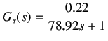
. It is as shown in figure 3.5 The figure 3.4 shows a screen shot of the same. We obtain $\tau$ = 78.92, K = 0.22. The transfer function obtained here is at the operating point of enterValue percentage of heat. If the experiment is repeated at a different operating point, the transfer function obtained will be different. The gain will correspondingly be more at a higher operating point. This means that the plant is faster at higher temperature. Thus the transfer function of the plant varies with the operating point. Let the transfer function we obtain in this experiment be denoted as

. We obtain

$\displaystyle G_s(s) = \frac{0.22}{78.92s+1}$ (3.12)

rokade 2017-04-23