Next: Procedure Up: Frequency Response Analysis of Previous: Conducting Sine Test on
Consider a sinusoidal input
| (4.1) |
The Laplace transform of the above equation yields
Consider the standard first order transfer function given below
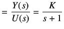 |
(4.3) |
Replacing the value of U(s) from equation 4.2, we get
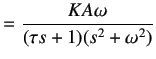 |
(4.4) | |
![$\displaystyle =\frac{KA}{\omega ^2\tau ^2 + 1}\left[\frac{\omega \tau ^2}{\tau s +1}- \frac{\tau s \omega}{s^2 + \omega^2}+\frac{\omega}
{s^2 + \omega^2}\right]$](img85.png) |
(4.5) |
Taking Laplace Inverse, we get
![$\displaystyle = \left[\frac {KA}{\omega^2\tau^2+ 1}\right]\left[\omega \tau e^{\frac {-t}{\tau}}-\omega \tau cos(\omega t)+
sin(\omega t)\right]$](img86.png) |
(4.6) |
The above equation has an exponential term
![]() . Hence, for large value of time, its value will
approach to zero and the equation will yield a pure sine wave. One can also use trigonometric identities to make the equation
look more simple.
. Hence, for large value of time, its value will
approach to zero and the equation will yield a pure sine wave. One can also use trigonometric identities to make the equation
look more simple.
![$\displaystyle = \left[\frac{KA}{\sqrt{\omega^2 \tau^2 + 1}}\right]\left[sin (\omega t) + \phi \right]$](img88.png) |
(4.7) |
where,
| (4.8) |
By observing the above equation, one can easily make out that for a sinusoidal input the output is also sinusoidal
but has some phase difference.
Also, the amplitude of the output signal, ![]() , has become a function of the input signal frequency,
, has become a function of the input signal frequency, ![]() .
.
 |
(4.9) |
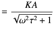
The amplitude ratio (AR) can be calculated by dividing both sides by the input signal amplitude A.
 |
(4.10) |
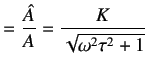
Dividing the above equation by the process gain K yields the normalized amplitude ratio ![]()
 |
(4.11) |
