Implementing PID Controller with Filtering using Backward Difference Approximation

Figure 5.12 shows Xcos diagram for implementing PID controller with filtering.

Figure 5.12: Xcos for PID controller with filtering available as pidN_virtual.xcos

PID filtered form is given by

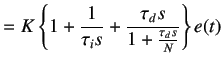$$u(t) =K\left\{1+\frac 1{\tau_i s}+\frac{\tau_d s}{1+\frac{\tau_d s}{N}}\right\}e(t)$$ (5.55)
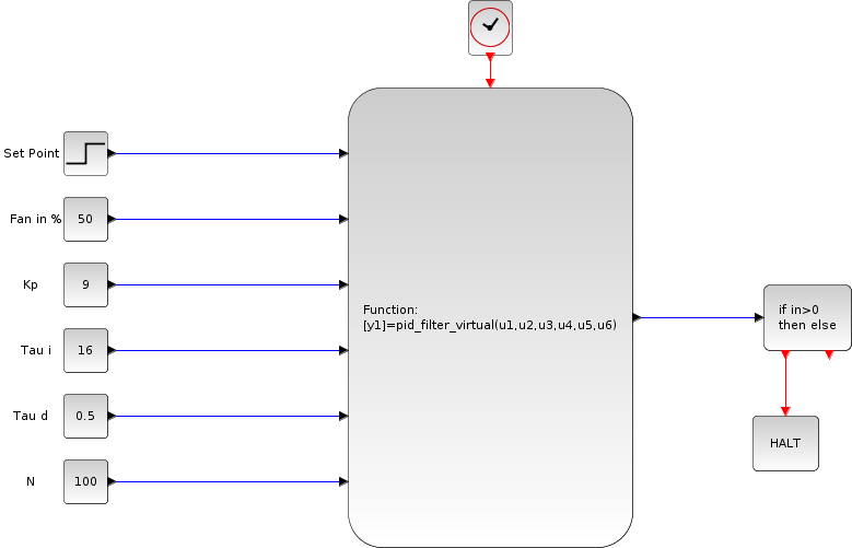
where N is large number of the order of 100. By maping controller given in equation 5.55 to the discrete time domain using backward difference formula, we get

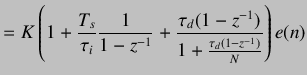$$u(n) =K\left(1+\frac{T_s}{\tau_i}\frac{1}{1-z^{-1}}+\frac{\tau_d (1-z^{-1})}{1+\frac{\tau_d(1-z^{-1})}{N}}\right)e(n)$$ (5.56)

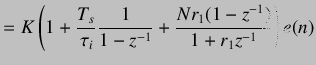$$u(n) =K\left(1+\frac{T_s}{\tau_i}\frac{1}{1-z^{-1}}+\frac{Nr_1(1-z^{-1})}{1+r_1z^{-1}}\right)e(n)$$ (5.57)
where

$$r_1 =-\frac{\frac{\tau_d}{N}}{\frac{\tau_d}{N}+T_s}$$ (5.58)
On cross multiplying, we obtain

$$(1-z^{-1})(1+r_1 z^{-1})u(n) =K[(1-z^{-1})(1+r_1 z^{-1})$$

$$+\frac{T_s}{\tau_i}(1+r_1z^{-1})+\frac{\tau_d}{T_s}(1-z^{-1})^2]e(n)$$ (5.59)
Simplifying and then by using shifting theorem, we obtain

$$u(n)+(r_1-1)u(n -1)$$

$$-r_1u(n -2)=K\left[1+\frac{T_s}{\tau_i}-Nr_1\right]e(n)$$

$$+K\left[r_1(1+\frac{T_s}{\tau_i}+2N)-1\right]e(n-1)$$

$$-K\left[r_1(1+N)\right]e(n-2)$$ (5.60)
Hence

$$u(n) =r_1u(n-2)-(r_1-1)u(n-1)$$

$$+s_0 e(n)+s_1e(n-1)+s_2e(n-2)$$ (5.61)
where

$$s_0 =K\left[1+\frac{T_s}{\tau_i}-Nr_1\right]$$ (5.62)

$$s_1 =K\left[r_1(1+\frac{T_s}{\tau_i}+2N)-1\right]$$ (5.63)

$$s_2 =-K\left[r_1(1+N)\right]$$ (5.64)