Determination of Second Order Transfer Function

In this section, we explore the efficacy of a second order model of the form

$$G(s) = \frac K{(\tau_1s+1)(\tau_2s+1)}$$ (2.12)

The response of the system to a step input of height $\Delta u$ is given by

$$y(s) = \frac K{(\tau_1s+1)(\tau_2s+1)} \frac{\Delta u}s$$ (2.13)

Splitting into partial fraction expansion, we obtain

$$y(s) = \frac K{\tau_1\tau_2} \frac 1 {\left(s+\dfrac 1{\tau_1}\right)\left(s+\dfrac 1{\tau_2}\right)}$$

$$= \frac A s + \frac B{s+\dfrac 1{\tau_1}} + \frac C{s+\dfrac 1{\tau_2}}$$

Through Heaviside expansion method, we determine the coefficients:

$$A = K$$

$$B = -\frac{K\tau_1}{\tau_1-\tau_2}$$

$$C = \frac{K\tau_2}{\tau_1-\tau_2}$$

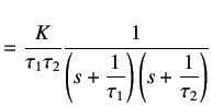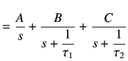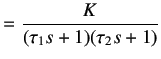
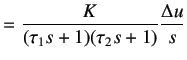
On substitution and inversion, we obtain

$$y(t) = K\left[ 1 - \frac 1{\tau_1-\tau_2} \left( \tau_1 e^{-t/\tau_1} - \tau_2 e^{-t/\tau_2} \right) \right]$$ (2.14)

We have to determine three parameters $K$, $\tau_1$ and $\tau_2$ through optimization. Once again, we follow a procedure identical to the first order model. The only difference is that we now have to determine three parameters. Scilab code
secondorder.sce calculates the gain and two time constants.