PI Controller using Trapezoidal Approximation

Figure 5.5 shows Xcos diagram for implementing PI controller.

Figure 5.5: Xcos for PI controller available as pi_ta_virtual.xcos

The PI controller in continuous time is given by,

$$u(t) =K \left\{e(t)+\frac{1}{\tau_i}\int_0^t e(t)dt\right\}$$ (5.13)
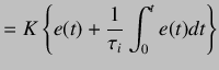
On taking the Laplace transform,we obtain

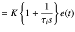$$u(t) =K\left\{1+\frac 1{\tau_i s}\right\}e(t)$$ (5.14)
By mapping controller given in equation 5.14 to the discrete time domain using trapezoidal approximation

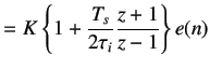$$u(n) =K\left\{1+\frac{T_s}{2\tau_i}\frac{z+1}{z-1}\right\}e(n)$$ (5.15)
On cross multiplying, we obtain

$$(z-1)u(n) =K\left\{(z-1)+\frac{T_s}{2\tau_i}(z+1)\right\}e(n)$$ (5.16)

$$z$$

$$u(n)-u(n-1) =K\left\{e(n)-e(n-1)+\frac{T_s}{2\tau_i}e(n)+\frac{T_s}{2\tau_i}e(n-1)\right\}$$ (5.17)
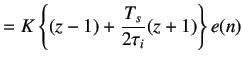
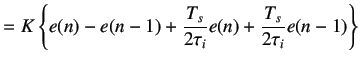
The PI controller is usually written as

$$u(n) =u(n-1)+s_0 e(n)+s_1e(n-1)$$ (5.18)
where

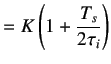$$s_0 =K\left(1+\frac{T_s}{2\tau_i}\right)$$ (5.19)

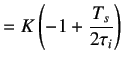$$s_1 =K\left(-1+\frac{T_s}{2\tau_i}\right)$$ (5.20)