Implementing PI Controller using Backward Difference Approximation

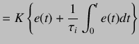$\displaystyle u(t)$	$\displaystyle =K \left\{e(t)+\frac{1}{\tau_i}\int_0^t e(t)dt\right\}$	(5.21)
On taking the Laplace transform, we obtain
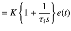$\displaystyle u(t)$	$\displaystyle =K\left\{1+\frac 1{\tau_i s}\right\}e(t)$	(5.22)
By mapping controller given in equation 5.22 to the discrete time domain using Backward difference approximation:
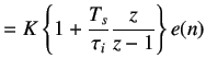$\displaystyle u(n)$	$\displaystyle =K\left\{1+\frac{T_s}{\tau_i}\frac{z}{z-1}\right\}e(n)$	(5.23)
On cross multiplying, we get
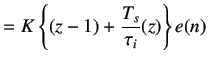$\displaystyle (z-1)u(n)$	$\displaystyle =K\left\{(z-1)+\frac{T_s}{\tau_i}(z)\right\}e(n)$	(5.24)
We divide by and then by using shifting theorem, we obtain
$\displaystyle u(n)-u(n-1)$	$\displaystyle =K\left\{e(n)-e(n-1)+\frac{T_s}{\tau_i}e(n)\right\}$	(5.25)
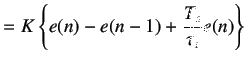
The PI controller is usually written as
$\displaystyle u(n)$	$\displaystyle =u(n-1)+s_0 e(n)+s_1e(n-1)$	(5.26)
where
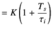$\displaystyle s_0$	$\displaystyle =K\left(1+\frac{T_s}{\tau_i}\right)$	(5.27)
$\displaystyle s_1$	$\displaystyle =-K$	(5.28)