Implementing PID Controller using Trapezoidal Approximation for Integral Mode and Backward Difference Approximation for the Derivative Mode

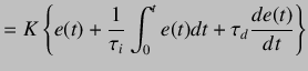$\displaystyle u(t)$	$\displaystyle =K \left\{e(t)+\frac{1}{\tau_i}\int_0^t e(t)dt+\tau_d\frac{de(t)}{dt}\right\}$	(5.46)
On taking the Laplace transform, we obtain
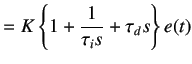$\displaystyle u(t)$	$\displaystyle =K\left\{1+\frac 1{\tau_i s}+\tau_d s\right\}e(t)$	(5.47)
By mapping controller given in equation 5.47 to the discrete time domain using trapezoidal approximation for integral mode and backward difference approximation for the derivative mode, we get
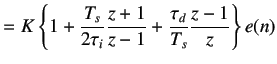$\displaystyle u(n)$	$\displaystyle =K\left\{1+\frac{T_s}{2\tau_i}\frac{z+1}{z-1}+\frac{\tau_d}{T_s}\frac{z-1}{z}\right\}e(n)$	(5.48)
On cross multiplying, we obtain
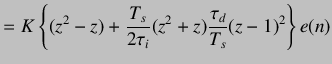$\displaystyle (z^2-z)u(n)$	$\displaystyle =K\left\{(z^2-z)+\frac{T_s}{2\tau_i}(z^2+z)\frac{\tau_d}{T_s}(z-1)^2\right\}e(n)$	(5.49)
We divide by and then by using shifting theorem, we get
$\displaystyle u(n)-u(n-1)$	$\displaystyle =K\left\{e(n)-e(n-1)+\frac{T_s}{2\tau_i}{e(n)+e(n-1)}\right.$
$\displaystyle \hspace{1cm}$	$\displaystyle + \left. \frac{\tau_d}{T_s}[e(n)-2e(n-1)+e(n-2)]\right\}$	(5.50)
The PID controller is usually written as
$\displaystyle u(n)$	$\displaystyle =u(n-1)+s_0 e(n)+s_1e(n-1)+s_2e(n-2)$	(5.51)
where
$\displaystyle s_0$	$\displaystyle =K\left[1+\frac{T_s}{2\tau_i}+\frac{\tau_d}{T_s}\right]$	(5.52)
$\displaystyle s_1$	$\displaystyle =K\left[-1+\frac{T_s}{2\tau_i}-2\frac{\tau_d}{T_s}\right]$	(5.53)
$\displaystyle s_2$	$\displaystyle =K\frac{\tau_d}{T_s}$	(5.54)