PID Controller

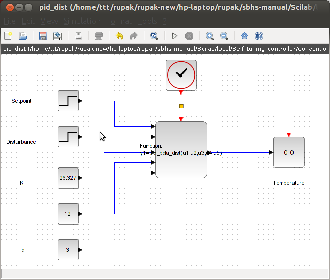
Figure 9.12: Xcos diagram for PID controller

The PID Controller in continuous time is given by

$$u(t) = K \left[e(t) + \frac 1{\tau_i}\int_0^t e(t)dt + \tau_d \frac{de(t)}{dt}\right]$$ (9.15)

On taking Laplace Transform, we obtain

$$u(s) = K \left[1 + \frac 1{\tau_i s} + \tau_d s\right]e(s)$$ (9.16)

By mapping equation 9.16 to discrete time interval by using the Trapezoidal Approximation for integral mode and Backward Difference Approximation for derivative mode, we get

$$u(n) = K \left[1 + \frac{T_s}{\tau_i} \frac{z}{z-1} + \frac{\tau_d}{T_s} \frac{z-1}{z}\right]e(n)$$ (9.17)

On cross multiplication, we obtain

$$(z^2-z)\times u(n) = K \left[(z^2-z) + \frac{T_s}{\tau_i} (z^2) + \frac{\tau_d}{T_s} (z-1)^2\right]e(n)$$ (9.18)

We divide by z, and using the shifting theorem, we obtain

$$u(n) - u(n-1) = K \left[e(n) - e(n-1) + \frac{T_s}{\tau_i} e(n) + \frac{\tau_d}{T_s}\left\{e(n) - 2e(n-1) + e(n-1)\right\}\right]$$ (9.19)

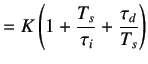
The PID Controller is usually written as

$$u(n) = u(n-1) + s_0 e(n) + s_1 e(n-1) + s_2 e(n-2)$$ (9.20)

where,

$$s_0 = K\left(1+ \frac{T_s}{\tau_i} + \frac{\tau_d}{T_s}\right)$$ (9.21)

$$s_1 =K\left[-1-2\frac{\tau_d}{T_s}\right]$$ (9.22)

$$s_2 =K\left[\frac{\tau_d}{T_s}\right]$$ (9.23)