Next: Experiments conducted to implement Up: Model Predictive Control in Previous: MPC theory
There are three main codes, which are being used for this experiment. mpc_init.sce is the code which opens the xcos window, wherein, we have step block for the set-point for temperature and the fan speed. Once the values have been entered into the xcos window and the simulation is started, the scifunc block of xcos calls the function mpc.sci after every sampling time. The mpc.sci in turn calls mpc_run.sci every time it is called by scifunc block. The mpc_run.sci code optimizes manipulated variable (heater) over control horizon and returns only the first manipulated variable (heater) value. This new heater value is then sent to the heater of the SBHS to control the temperature at the set point.
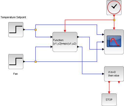
When mpc_init.sce is executed in scilab, an xcos window opens up. The xcos window has two step input blocks. The first step input block on the left side, is for the Temperature set point and the second step input block is for the fan (disturbance variable). Also the sampling time can be entered via clock block present on the xcos.
For all the experiments done for this project, sampling time of 1 second was used (entered via clock block of xcos).
Refer to the figure below for a clear picture of the xcos.
Other codes that were used other than mpc_run.sci for conducting this experiment are mpc_init.sce and mpc.sci. Both these codes were originally taken from Moodle (Process controls course for SBHS assignment). Please note that, both these codes were slightly modified to work with our MPC.
The only changes done in the original codes are:
rokade 2017-04-23