Next: 2-DOF Pole Placement Controller Up: 2-DOF Controller theory and Previous: 2-DOF Controller theory and
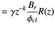
We want the desired output, ![]() , of the system to be related to the setpoint
, of the system to be related to the setpoint ![]() in the following manner:
in the following manner:
 |
(6.14) | |
|
| ||
 |
(6.15) | |
|
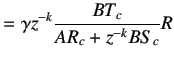
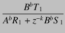
Simplifying the block diagram shown in figure 6.3 yields
| ||
 |
(6.16) | |
|
We have dropped the argument of
| ||
 |
(6.17) | |
|
We can expect some cancelations between the numerator and the denominator polynomials in the LHS, thereby making
| ||
| (6.18) | ||
| (6.19) | ||
| (6.20) | ||
| (6.21) |
Hence, equation 6.17 becomes
 |
(6.22) | |
|
After cancelling out the common factors, we obtain
| ||
 |
(6.23) | |
|
We obtain,
| ||
| (6.24) | ||
| (6.25) | ||
|
Equation 6.26 is known as the Aryabhatta's identity and can be used to solve for
| ||
| (6.26) | ||
|
The expression for
| ||
 |
(6.27) | |
|
and the desired closed loop transfer function will be
| ||
 |
 |
(6.28) |
