2-DOF Pole Placement Controller Design and Implementation using SBHS

We obtain a first order transfer function of the plant using the step test approach. Refer to the chapter on Step Test using SBHS for more details. The model obtained is

$\displaystyle G(s)$ $\displaystyle =\frac{0.42}{35.61s+1}$ (6.29)

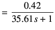
with a time constant of
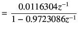
 $ \tau = 35.6 s$ and gain $ K=0.42$. After discretization with sampling time = 1 s, we obtain


$\displaystyle G(z)$ $\displaystyle =\frac{0.0116304z^{-1}}{1-0.9723086z^{-1}}$ (6.30)

Refer to the Scilab code myc2d.sci 6.1. We shall now define good and bad factors as

$\displaystyle A^g$ $\displaystyle =1-0.9723086z^{-1}$    
$\displaystyle A^b$ $\displaystyle =1$    
$\displaystyle B^{g}$ $\displaystyle =0.0116304$    
$\displaystyle B^{b}$ $\displaystyle =1$    

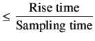
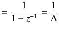
Let us now define the transient specifications. We choose Rise Time =100 s and Overshoot ($ \epsilon$)= 5%. Number of samples in one rise time ($ N_r$), [1], is calculated as


$\displaystyle N_r$ $\displaystyle \le\frac{\text{Rise time}}{\text{Sampling time}}$    
  $\displaystyle =100$    
% latex2html id marker 12347
$\displaystyle \therefore, \omega$ $\displaystyle =\frac{\pi}{2N_r}$    
  $\displaystyle =0.015708$    

and


$\displaystyle \rho$ $\displaystyle \le \epsilon ^{\omega / \pi}$    
  $\displaystyle =0.98513$    

The closed loop characteristic polynomial is given by,


$\displaystyle \phi _{cl}$ $\displaystyle = 1-2\rho cos\omega z^{-1} + \rho ^2z^{-2}$    
  $\displaystyle =1-1.9700229z^{-1}+0.9704870z^{-2}$    

Refer to the Scilab code desired.sci to calculate $ N_r$, $ \omega$, $ \rho$ and $ \phi_{cl}$. The code is available in the same location as myc2d.sci. But according to equation 6.26,


$\displaystyle A^bR_1+z^{-k}B^bS_1$ $\displaystyle =\phi_{cl}$    

Recall that we have not considered external disturbance in the block diagram shown in figure 6.3. However, we can still up to some extent take care of the disturbances. This is achieved by using the Internal Model Principle. If a model of step is present inside the loop, step disturbances can be rejected [1]. We can apply this by forcing $ R_c$ to have this term. A step model is given by


$\displaystyle 1(z)$ $\displaystyle =\frac{1}{1-z^{-1}} = \frac 1{\Delta}$    

Therefore,


$\displaystyle R_c$ $\displaystyle =B^g\Delta R_1$    

$ \Delta$ has a root which lies on the unit circle. Hence it has to be treated as a bad part and should not be canceled out. Hence, we should make sure that all of the occurrences of $ R_1$ have this term.


Therefore,

$\displaystyle \phi _{cl}$ $\displaystyle =A^b\Delta R_1+z^{-k}B^bS_1$ (6.31)

Hence,


$\displaystyle A^b\Delta R_1+z^{-k}B^bS_1$ $\displaystyle =1-1.9700229z^{-1}+0.9704870z^{-2}$ (6.32)

is expression is known as the Aryabhatta Identity and is solved using rigorous matrix calculations. The explanation of this operation is not considered here. Refer to [1] for more details on Aryabhatta's Identity. Refer to the Scilab code pp_im.sci, which is used to split the denominator and numerator polynomials of the plant transfer function into good and bad factors, and solving the Aryabhatta's Identity given in equation 6.33. On solving equation 6.33, we get

$\displaystyle R_c$ $\displaystyle =0.0116304-0.0229175z^{-1}+0.0112871z^{-2}$    
$\displaystyle S_c$ $\displaystyle =0.0004641-0.0004512z^{-1}$    
$\displaystyle T_c$ $\displaystyle =1-0.9723z^{-1}$    
$\displaystyle \gamma$ $\displaystyle =0.0004641$    

All the above calculations are incorporated into a single Scilab code named twodof_para.sce 6.2.


Subsections
rokade 2017-04-23