Next: 2-DOF Controller Design using Up: Two Degrees of Freedom Previous: Two Degrees of Freedom
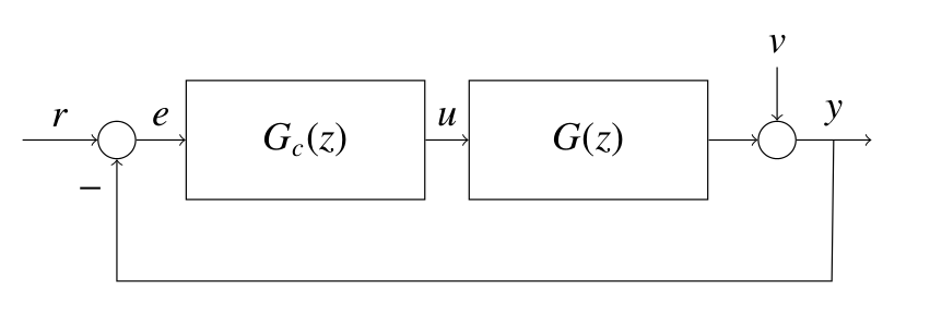
A feedback control strategy is shown in figure 6.1. The reference ![]() and the output
and the output ![]() are continuously compared
to generate error
are continuously compared
to generate error ![]() , which is fed to the controller
, which is fed to the controller ![]() , to take appropriate control action.
, to take appropriate control action. ![]() is the controller
output that is fed to the plant. Unlike feed forward controllers, exact knowledge of the plant
is the controller
output that is fed to the plant. Unlike feed forward controllers, exact knowledge of the plant ![]() and the disturbance
and the disturbance
![]() is not necessary in this case. Feedback controllers are further classified as One Degree of Freedom (1-DOF) controllers
and Two Degrees of Freedom (2-DOF) controllers. Degree of freedom refers to the number of parameters that are free to vary
in a system. A higher degree of freedom controller makes the plant less susceptible to disturbances.
is not necessary in this case. Feedback controllers are further classified as One Degree of Freedom (1-DOF) controllers
and Two Degrees of Freedom (2-DOF) controllers. Degree of freedom refers to the number of parameters that are free to vary
in a system. A higher degree of freedom controller makes the plant less susceptible to disturbances.
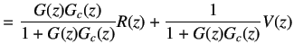
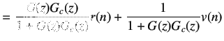
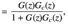
The expression for output, ![]() of the system shown in figure 6.1 is given by
of the system shown in figure 6.1 is given by
 |
(6.1) |
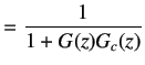
 |
(6.2) | |
|
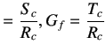
Let,
| ||
 |
(6.3) | |
 |
(6.4) | |
|
Therefore,
| ||
| (6.5) | ||
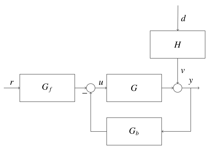
A Two Degrees of Freedom controller is as shown in figure 6.2. Here, ![]() and
and ![]() together
constitute the controller.
together
constitute the controller. ![]() is in the feedback path and is used to eliminate the effect of disturbances,
whereas
is in the feedback path and is used to eliminate the effect of disturbances,
whereas ![]() is in the feed forward path and is used to help the output track the reference input.
is in the feed forward path and is used to help the output track the reference input.
The expression for control effort ![]() in figure 6.2 is given by
in figure 6.2 is given by
| (6.6) | ||
|
Let
| ||
 |
(6.7) | |
|
where
| ||
| (6.8) | ||
|
Consider a plant whose model is given by
| ||
| (6.9) | ||
|
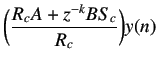
Substituting equation 6.8 in equation 6.9, we get
| ||
![$\displaystyle =z^{-k}\frac{B}{R_c}\bigg[T_cr(n)-S_cy(n)\bigg]+v(n)$](img257.png) |
(6.10) | |
|
Solving for
| ||
 |
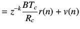 |
(6.11) |
|
This can also be written as
| ||
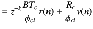 |
(6.12) | |
|
where
| ||
| (6.13) | ||
We want the following conditions to be satisfied while designing a controller.
 must be close to unity, so that reference tracking is achieved